The stereophonic zoom

A variable dual-microphone system for stereophonic sound recording

By Michael Williams

Introduction

In the field of monophonic sound recording, the sound recording engineer has a large range of different types of microphones from which to choose his particular preference for recording any specific sound source or sound environment. All manner of frequency response curves can be chosen either to modify the timbre of the sound source, or, if desired, to reproduce it as faithfully as possible. The directivity of the microphone and its position in relation to the source can also be chosen to obtain, fairly easily, the desired relationship of direct to reverberant sound.

Unfortunately, we do not have the same flexibility in the choice of microphone systems for stereophonic sound recording. The number of available microphone systems and the types of microphones used is relatively limited, and, almost without exception, those that are available have fixed characteristics. It is undeniable that each of these systems may be optimum in one particular situation, however, none of them can be considered as meeting all our needs for stereophonic sound recording.

In no way can we consider our present stereophonic sound recording microphone systems as enabling the listener to experience a natural perception of the original sound source. The sound image as perceived by the listener is conditioned by the choices imposed by the sound recording engineer. Balance, sound perspective, localisation, etc are determined by the sound engineer, and his or her skill in transmitting these parameters to the listener will remain part of the art of sound recording for many years to come.

It is unfortunately too often the case that the position of the microphone system is a compromise between a good stereophonic sound image and the optimum ratio of direct to reverberant sound. In more general terms, it is evident that the different parameters that must be taken into account during the process of sound recording are infinitely variable, each situation encountered being in itself unique. The conditions that are necessary to achieve optimum results in a specific context with the present “tools of the trade” are rarely encountered.

Even in the face of this very limited choice, many attempts have been made to establish which, of the different systems available, could be considered as having the best overall performance. The futility of this type of approach becomes immediately evident in light of the fact that each specific system has a unique set of characteristics and that the sound recording sources and environment are infinitely variable.

On the contrary, rather than reduce the choice of systems, an effort must be made to increase the number of systems available. Each sound recording engineer must have the largest possible selection of systems to choose from, in order to solve the specific problems presented by a particular recording situation and, to express his or her own personal interpretation, as freely as possible.

The ideal is of course an infinitely variable system covering all situations. This document describes just such a variable dual microphone system called « The Stereophonic Zoom » and explains the basic theory of dual microphone systems in general and how this has been interpreted to develop this variable system.

The “Stereophonic Zoom” enables the sound recording engineer to get much nearer to the optimum result in the great majority of recording environments. It uses any desired first-order microphone directivity with its associated frequency response curve and enables reasonably independent control of:

• Stereophonic Recording Angle

• Angular or Geometric Distortion

• Reverberation distribution

• Early reflection localisation

The analysis of the physics and psychoacoustics involved in this type of system has already been published in papers given by the author to various Conventions of the Audio Engineering Society:

1984 – 75th AES Convention in London – Preprint 2072, “Stereophonic Zoom; a practical approach to determining the characteristics of a spaced pair of microphones”

1987 –  82nd AES Convention in London – Preprint 2466, “Unified Theory of Microphone Systems for Stereophonic Sound Recording”

1990 – 88th AES Convention in Montreux – Preprint 2931, “Operational limits of the Variable M/S Stereophonic Microphone System”

1991 – 91st AES Convention in New York – Preprint 3155, “Early Reflections and Reverberant Field Distribution in Dual Microphone Stereophonic Sound Recording Systems”

The basic operational simplicity of this system is described in this document. This should enable the sound recording engineer quickly to use the St Zoom System for everyday sound recording with a minimum of study.

The operational approach

I. 1  Characteristics of the standard listening configuration

The basic characteristics of a stereophonic sound recording system are determined as a function of the relative position of the loudspeakers in relation to the listener during reproduction. It is almost universally accepted as a Standard Listening Configuration that the listener must be placed at the summit of an equilateral triangle, the loudspeakers being positioned at each extremity of the base of the triangle and directed towards the listener (Figure 1).

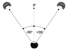Figure 1 – Standard listening configuration[/caption]

It is essential to attenuate reflections from the ceiling, floor and walls and, in addition, symmetry should be maintained in relation to the shape of the listening room so that any remaining reflections affect equally the sound heard from the left and right channels. Only then will the conditions be adequate to hear with clarity and precision the stereophonic image generated by the specific microphone system used during the recording session.

Further improvements can be made to the listening environment by following the IEC recommendations concerning the specification of a standard listening room. Another interesting solution to the problems in designing a listening room has been developed by Bob Walker of the BBC Research Dept., and published in Audio Engineering Society Preprints 3543, 3853 and 4645.

I.  2 Localisation

Without going into all the details described in Chapter II, one can say that the localisation of a sound source between the loudspeakers is obtained:

• by varying the intensity ratio between the two loudspeakers

• or by creating a time difference between them

• or by a combination of both intensity and time difference

If the same sound is produced by each loudspeaker at the same level and at the same instant, then one will get the impression that the sound image is situated in the centre between the two loudspeakers (0° in Figure 1). If on the other hand, the sound produced by the right channel is louder than the left, then the localisation of the sound image will be situated somewhere to the right-hand loudspeaker (between 0° and 30° in Figure 1). If on the other hand, the sound intensity of both channels is the same, but there exists a small time difference (less than a millisecond) between each channel then a similar effect is obtained, i.e., if the left channel is in advance of the right, then the sound is localised to the left, and vice versa.

It is quite commonplace to create a variation of the Intensity Ratio on a mixing desk, by means of a simple potentiometer, normally called a “pan pot”. On the other hand, it is quite exceptional to find a variable delay line associated with a mixing desk to create Time Difference information between the left and right channels. Both of these techniques produce localised sound sources between the loudspeakers, unfortunately without any information necessary to produce natural acoustic size and stereophonic acoustic environment. This process is very aptly called in French “Monophonie Dirigé”, which translates to “Directed Monophony” or “Positioned Monophony”, as opposed to Natural Stereophony. Even the word “Natural” in this context could be considered a misnomer, as we are really involved in the process of producing the “impression” of a natural listening experience.

The intention of this document is to describe a variable dual microphone system that will reproduce realistic stereophony, thereby creating a good “impression” of relative acoustic size for each sound source and maintaining the continuity of the sound environment. It is important again to emphasise the word “impression” in this context, as we are indeed only concerned with impressions. For instance, in recording an orchestra, we must create the impression of depth and localisation of individual instruments, as realistically as possible. The acoustic signals, received by our ears in the listening room coming from the loudspeakers, bear very little relation to the acoustic information actually received by the listener in the concert hall. In fact, it could be said that any recording and reproduction system which is capable of giving this “impression” is acceptable, no matter what means are used to obtain it.

Intensity Difference (or Intensity Ratio) and Time Difference information can be generated by two spaced directional microphones. The Intensity Difference information generated by the microphones is a function of the position of the sound source and the angle between the axes of the directivity patterns of the microphones. The Time Difference information, on the other hand, is a function of the position of the sound source and the distance between the microphones. To obtain Intensity Difference information only, the microphones must be “coincident”, whilst Time Difference information only will be obtained with spaced omnidirectional microphones or parallel-spaced directional microphones.

I.  3. 1  Operational characteristics of the variable dual-microphone system

A Variable Dual-Microphone System is basically two identical directional microphones mounted in such a way as to be able to modify both the distance between the microphone capsules and the angle between the axis of directivity (Figure 2).

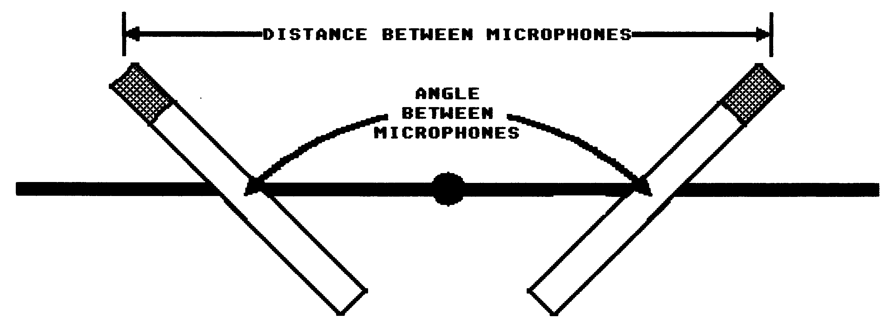Figure 2 – Angle and distance between two microphones

The distance and angle between the microphones is chosen according to the Stereophonic Recording Angle that is desired. Figure 3 shows the various combinations of distance and angle as a function of the Stereophonic Recording Angle. The x and y axes (abscissa and ordinate) represent the Distance and Angle between the microphones, whereas the individual curves represent the various combinations of angle and distance needed to obtain a specific stereophonic recording angle (shown in circles as a ± value on the diagrams).

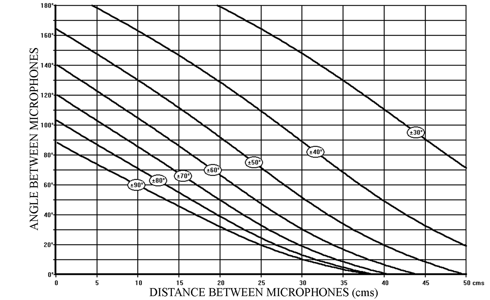Figure 3 – SRA diagram for cardioid microphones

From now on, this diagram, which we will call the “SRA diagram” (Stereophonic Recording Angle diagram), is our basic guide to choosing a specific combination distance/angle corresponding to a given Stereophonic Recording Angle. Certain limitations to our choice of distance/angle will be considered a little later in this chapter.

The Stereophonic Recording Angle is defined as:

THAT SECTOR OF THE SOUND FIELD IN FRONT OF THE MICROPHONE SYSTEM WHICH WILL PRODUCE A VIRTUAL SOUND IMAGE BETWEEN THE LOUDSPEAKERS.

Let us consider as an example, the combination:

               20cm / 90°
(20cm between the microphone capsules / 90° angle between the directivity axes)

We can read from the SRA diagram (Figure 3) that this combination has an S.R.A. of:

               ± 50°

Note: The Stereophonic Recording Angle is, by convention in this publication, always specified as ± an angle, ‘+’ indicating clockwise measurement and ‘-‘ indicating anticlockwise measurement. This convention is adopted in order to avoid confusion with the specification of the angle between the microphones which is specified as the total angle. In the above example this means that + 50° is measured clockwise from the front centre axis of the microphone system, and -50° measured anticlockwise (a total stereophonic coverage angle of 100°).

Two other possible combinations with the same Stereophonic Recording Angle of ± 50° are:

               10 cm / 130° and 30 cm / 50°

But of course, there is a multitude of combinations possible for a specific SRA. Here are two examples of other readings from the SRA diagram:

               10cm / 60° has an SRA of ± 90°

               40cm / 110° has an SRA of ± 30°

All sound sources within this angular sector will be reproduced as virtual sound sources BETWEEN the left and right loudspeakers. Any sound source outside this sector will be reproduced ON either one or the other loudspeaker. The operational procedure for setting up the system consists basically of measuring the sector occupied by the sound source and using this as the required SRA of the microphone system. The combination distance/angle can then be read from the SRA diagram.

It should be said, however, that it is not obligatory for the SRA to be equal to the angle occupied by the sound source. Most sound recording engineers in fact prefer the SRA to be slightly larger than the sound source sector. This is equivalent to leaving a little headroom in a picture or more correctly in this case “sideroom” in the sound image. The amount of sideroom is obviously a matter of individual judgement but is rarely more than about 10° for a small group of musicians. On the other hand, in the case of a much larger orchestra, it is quite often necessary to do the opposite and place the limits of the SRA within the orchestra (negative sideroom), the left limit being within the first violins, the right limit within the double basses. This allows more space for the individual instruments (flute, clarinet, oboe, etc.) in the middle of the orchestra. But this is a question of individual preference, and there are as many different choices as there are sound recording engineers!

I. 3. 2 Microphone position

How does one determine the position of the microphone in the first place? This is not a question of measurement or even following a set of rules, but more one of individual preference. However, it is simple enough to describe those factors that are modified with a change in microphone position.

The variation of distance between the sound source and the microphone will certainly change the level of direct sound reaching the microphone, however, this will be perceived as a change in the ratio of direct to reverberant sound. It is this ratio that is responsible almost entirely for our perception of depth or sound perspective within the sound image. Each individual sound engineer will have his or her own subjective appreciation of the optimum value of this ratio in relation to the type of recording being made. In the case of multiple sound sources, for instance, with an orchestra, the position of the microphone system must also take into account the relative acoustic levels of individual instruments or sections of instruments, the aim being to obtain a good “balance” between all the different sections of the orchestra.

Once the microphone position has been determined, one has only to measure the angular sector covered by the whole of the orchestra, decide how much “sideroom” one wishes, and then read off the corresponding combination of distance and angle:

Stereophonic Recording Angle  = Sound Source Sector + “Sideroom”

I.  3. 3  Frequency response curve and directivity

A major advantage of using the « Stereo Zoom » or “Variable Dual-Microphone System” is that we do not need to restrict the choice of directivity patterns to only cardioid microphones. In Figure 4, the SRA Diagram is shown for a specific Hypocardioid (“Wide Angled cardioid” or ” Infra-carded”) Microphone, and Figure 5 shows the SRA Diagram for a specific Hypercardioid Microphone.

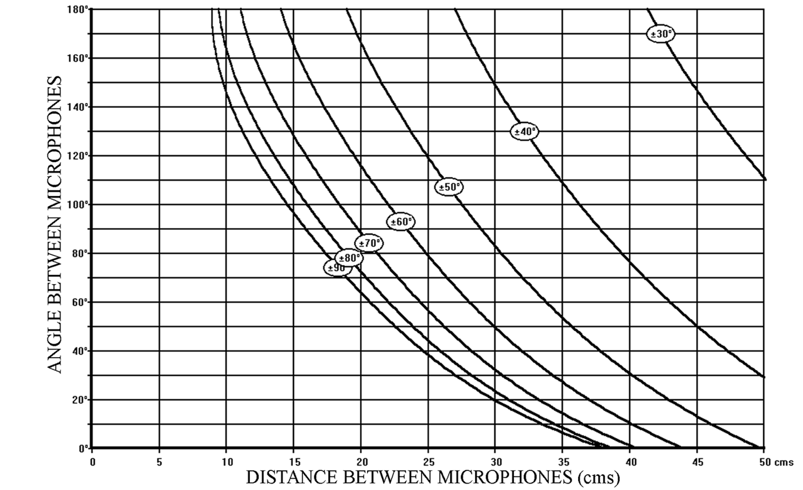Figure 4 – SRA diagram for a hypocardioid microphone (back attenuation 10 dB) 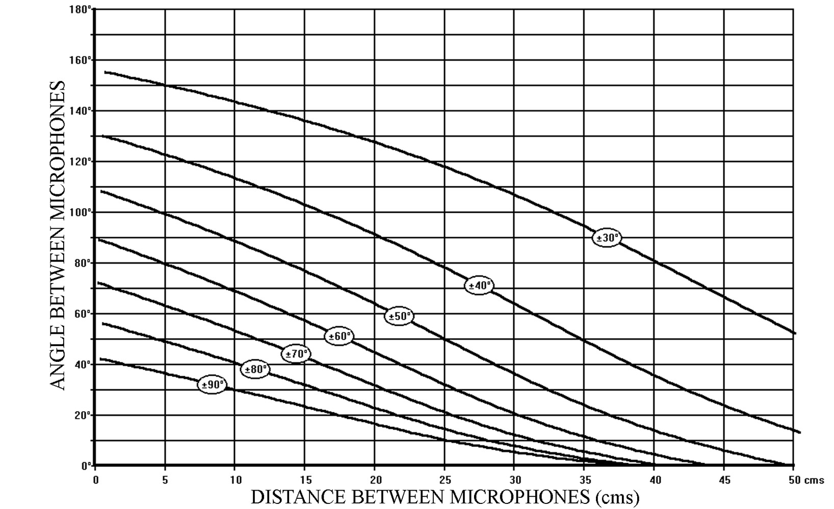Figure 5 – SRA diagram for a hypercardioid microphone (back attenuation 10 dB)

It is general practice to use omnidirectional microphones to generate “Time Difference only” stereophony.  However, by reducing the angle between two directional microphones to 0° and by varying only the distance between the microphones the same result is obtained. The fact that the two microphones are parallel means that, although there is attenuation due to the directivity of the microphone when the sound source is to one side or the other of the microphone axis, the attenuation is the same on both microphones. Therefore no “Intensity Difference” information is generated. This means that the SRA values can be read off any of the SRA diagrams as long as the angle between the microphones is considered to be 0°. This is more easily seen in Figure 4 – the SRA diagram for a hypocardioid directivity pattern. For example:

               35cm produces an SRA of ± 90°

               41cm ————————- ± 70°

               50cm ————————- ± 50°

These values can be verified in Figure 6, which represents the SRA Diagram for Omnidirectional Microphones. Variation in the angle between the microphones will obviously not produce any change in the Stereophonic Recording Angle of a specific microphone system, as long as the microphones have a truly omnidirectional response over the major part of the audible spectrum.

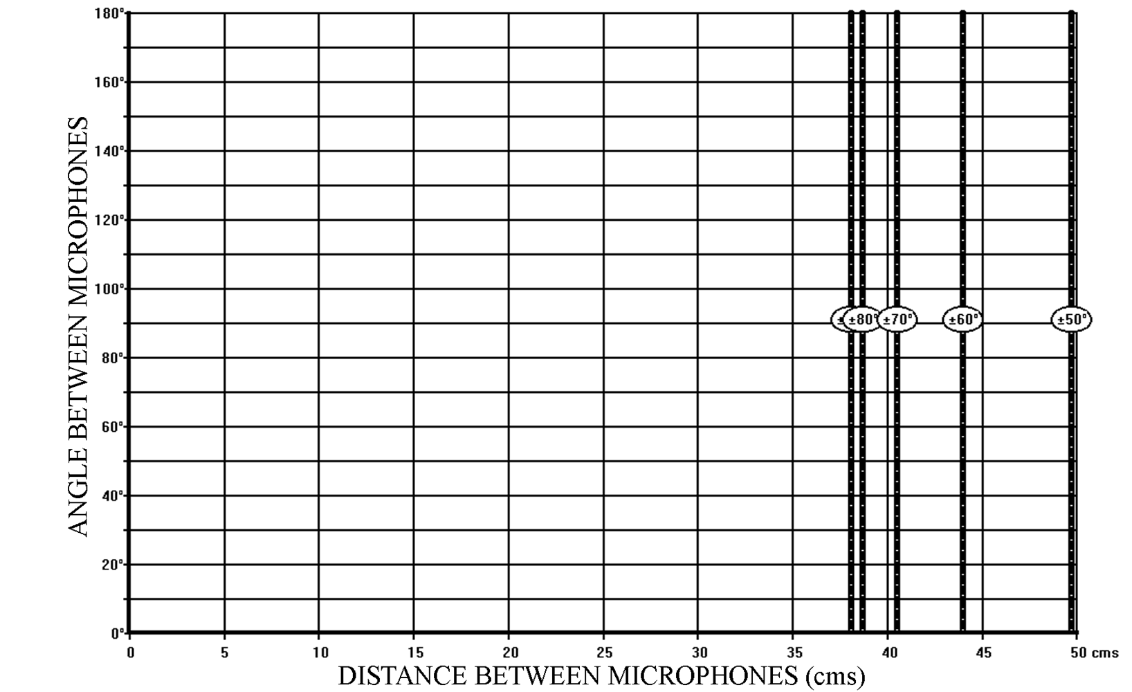Figure 6 – SRA diagram for omnidirectional microphones

However, there are other important factors that must influence our choice of directivity pattern for the microphones. The first consideration is the frequency response curve associated with a specific directivity. Omnidirectional microphones have in general a good response in the bass frequencies. In the case of omnidirectional electrostatic microphones, the frequency response can go as low as a few Hertz. However, this is not the case for pressure gradient microphones: a figure-of-eight microphone has a 6dB/octave roll-off in the bass frequencies. The exact frequency at which the roll-off starts is determined by the manufacturer, depending upon the required microphone sensitivity and signal-to-noise ratio. Figure 7 shows the variation in roll-off as one passes from omnidirectional through to figure-of-eight directivity. This series of frequency response curves related to directivity assumes that all other frequency-dependent factors are equal, especially sensitivity.

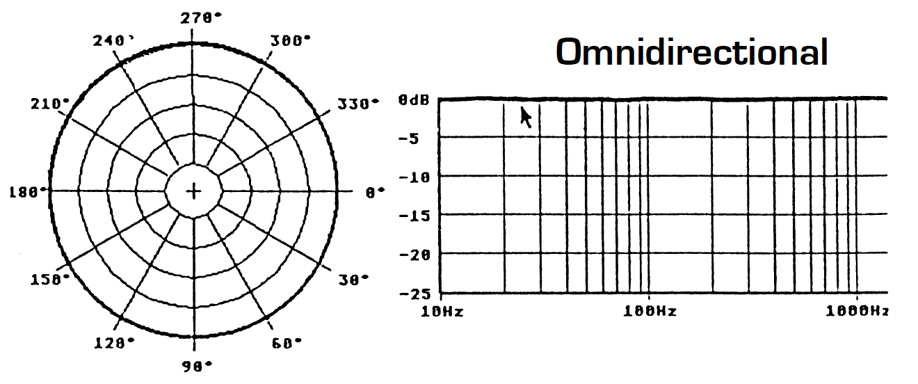
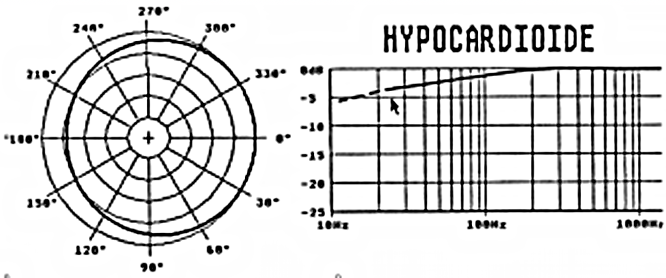
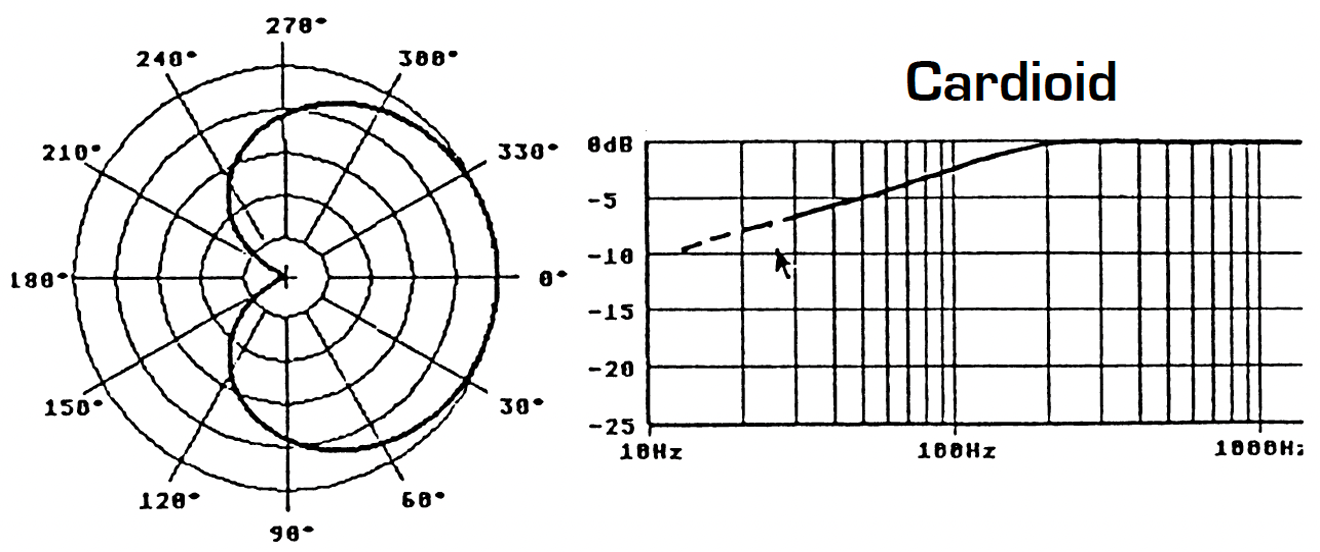
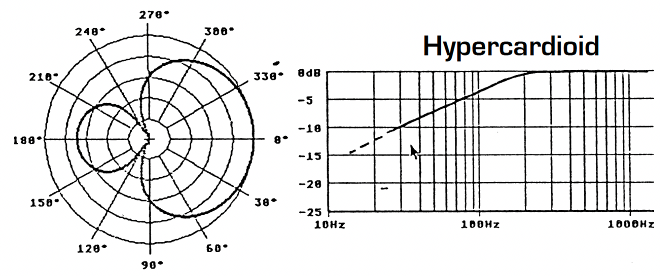
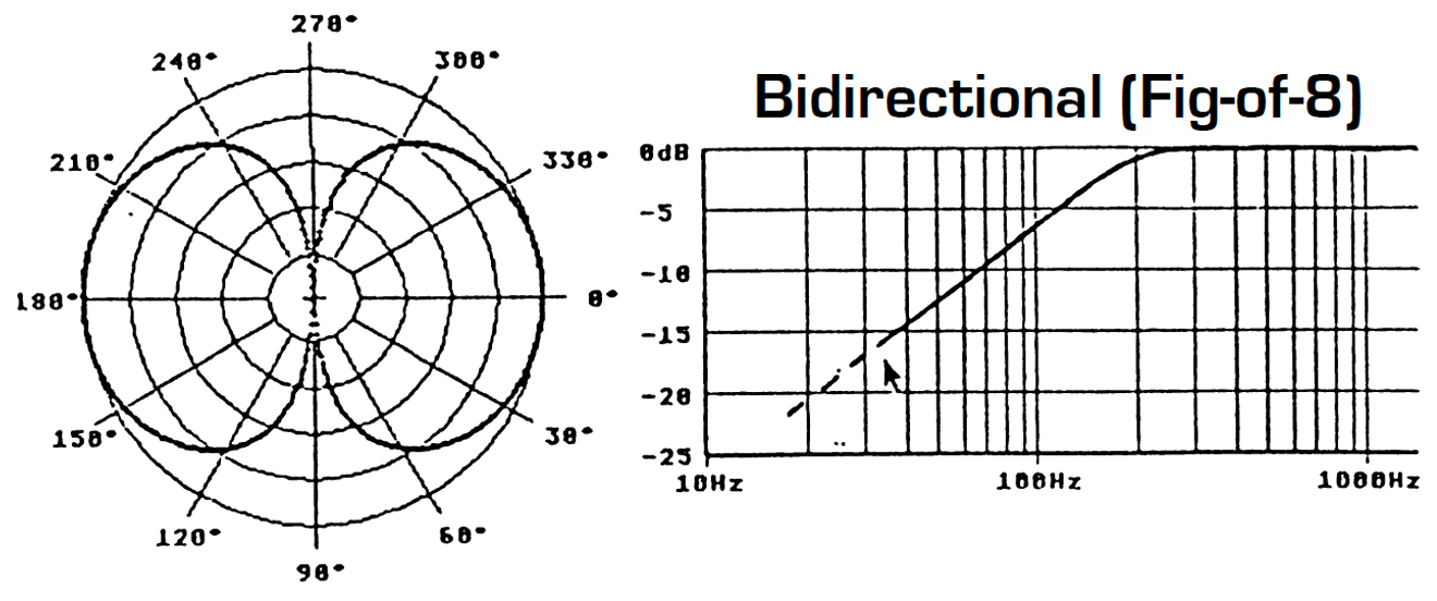Figure 7 – Frequency response curve and directivity

It is therefore quite possible to take advantage of the better bass response with a hypocardioid microphone as against a cardioid, or on the contrary, to attenuate bass response with a hypercardioid. This choice is generally determined by the acoustic environment of the recording (traffic or ventilation noise, structure-born vibration, etc…), or simply by one’s personal preferences. However, any practical Stereophonic Recording Angle (between ± 90° and ± 30°) can be obtained with any chosen directivity pattern. Other reasons for choosing different directivity patterns will be considered in later chapters, for example, the response of the microphone system to the surrounding acoustic environment.

I. 4 Operational limitations

In Figures 3, 4 and 5 it would seem that there is an almost infinite choice of the different combinations of distance and angle that produce a given Stereophonic Recording Angle. Although this is certainly the case concerning the angular limits of the Stereophonic Recording Angle, there are however some other operational limitations which must be taken into account in the final choice of a microphone system. Two additional major characteristics of the reproduced stereophonic sound field must be considered:

• Distortion of Angular Localisation within the reproduced sound field

• Variation of the ratio of direct to reverberant sound within the reproduced sound field

A more detailed analysis of these two characteristics will follow in paragraph I. 4.1 and I. 4.2. The SRA Diagrams represented in Figures 3, 4 and 5 are just the first stage in the complete graphical representation of the characteristics of different microphone systems. A quick look at Figures 8, 9 and 10 will show the method now used to represent these two additional characteristics:

• The values of Angular Distortion are represented within a square box on each curve

• The two shaded areas at the top and the bottom of each diagram show the combinations where the ratio of direct to reverberant sound varies within the stereophonic recording angle. In the top-shaded area, there is too much reverberation in the centre zone of a particular microphone system, whereas in the bottom-shaded area the reverberation increases towards the extremities of the SRA.

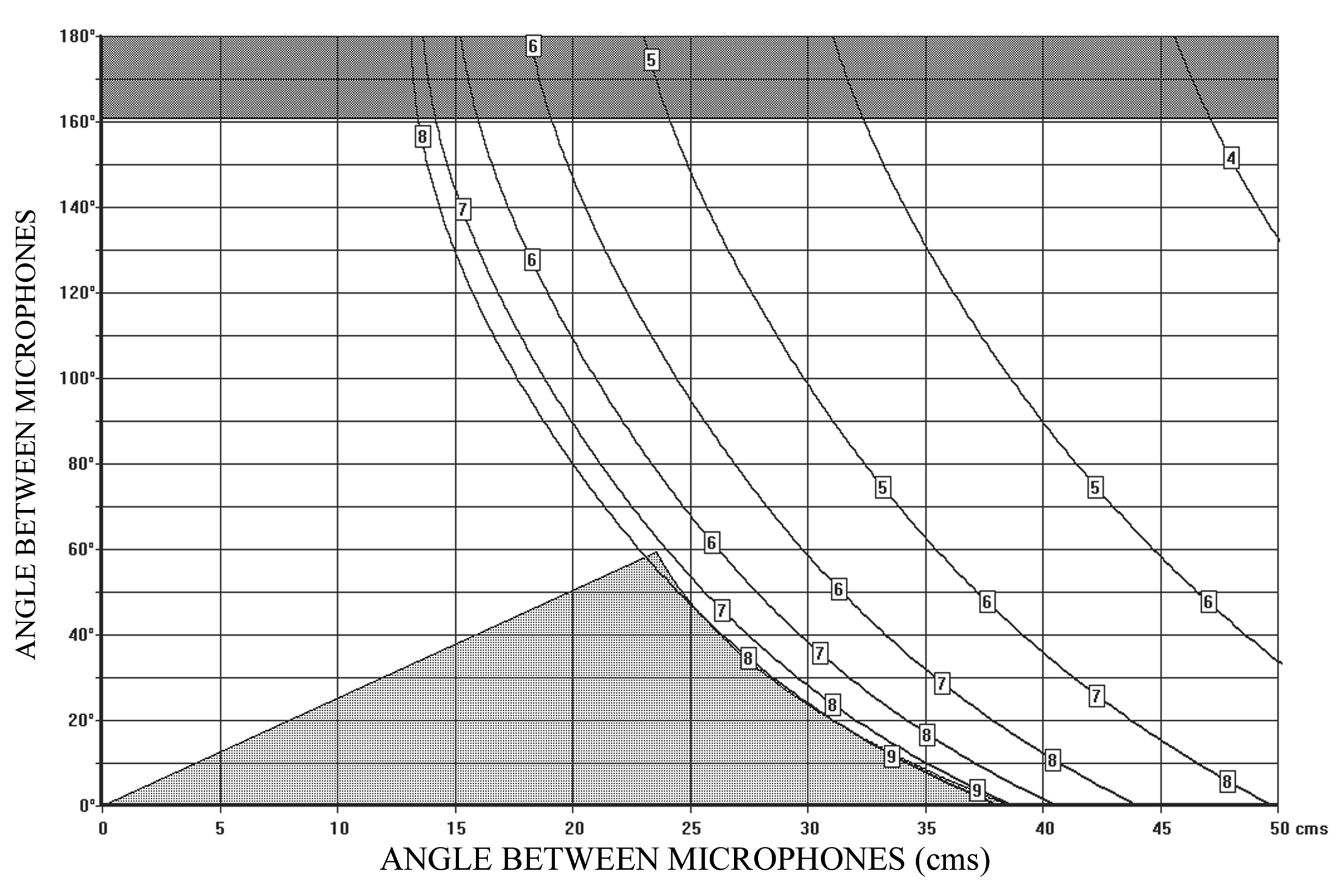Figure 8 – SRA diagram for hypocardioid microphones (back attenuation 10dB) showing angular distortion and reverberation limits 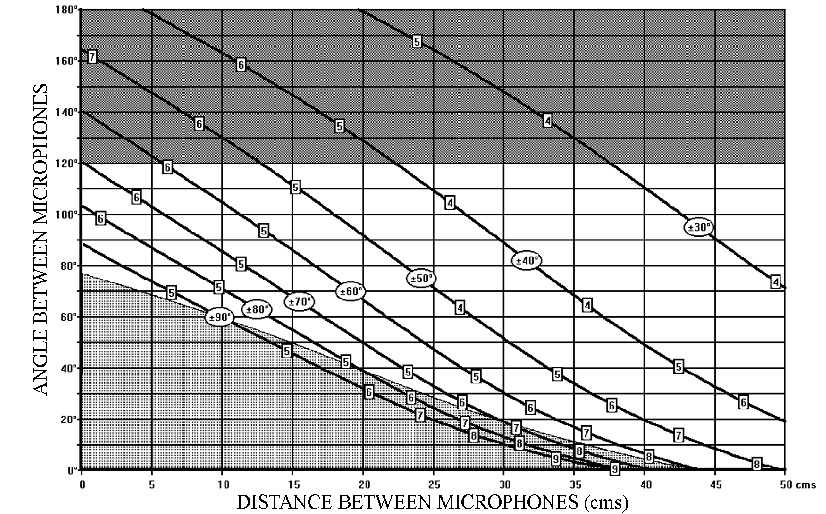Figure 9 – SRA diagram for cardioid microphones showing angular distortion and reverberation limits 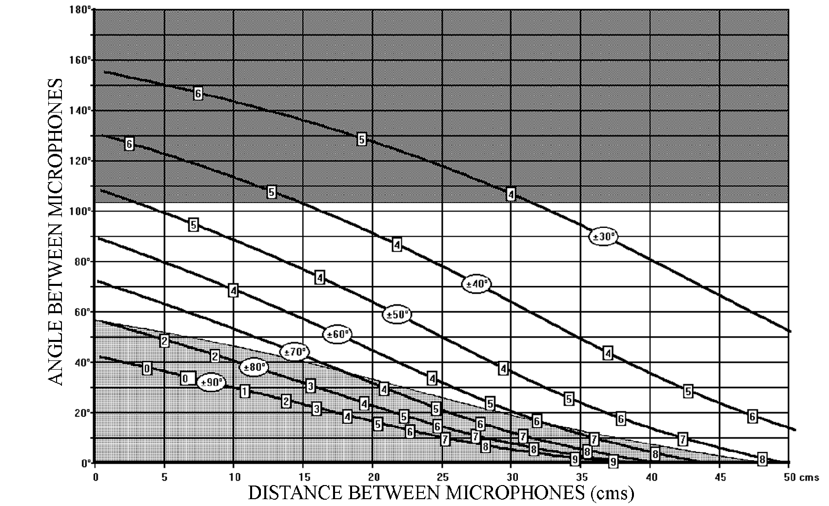Figure 10 – SRA diagram for hypercardioid microphones (back attenuation 10 dB) showing angular distortion and reverberation limits

I.  4.1 Angular distortion – geometric distortion

The characteristic of Angular Distortion or Geometric Distortion describes the variation of the position of each particular element of the sound source within the reproduced sound stage. It has nothing to do with the characteristic of electronic distortion of the signal. Angular Distortion represents the angular linearity of reproduction, that is the relative angular position of individual sound sources within the Stereophonic Recording Angle when reproduced in front of the listener.

The characteristic of Angular Distortion, for a given dual microphone system also must not be confused with the Angular Compression or Expansion of the reproduced sound stage in relation to the original sound field. The sound source normally occupies a sector that is a good deal larger than the 60° reproduced in the equilateral triangle listening situation, therefore angular compression of the reproduced sound source must exist (Figure 11).

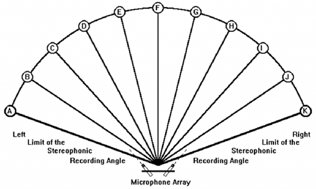
Figure 11 – Angular compression in reproduction (but without angular distortion)

The opposite situation (shown in Figure 12), in which the sound source sector is less than 60°, is the situation in which expansion of the angular proportions of the reproduced sound image occurs, but this situation is hardly ever encountered.

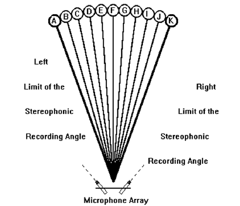
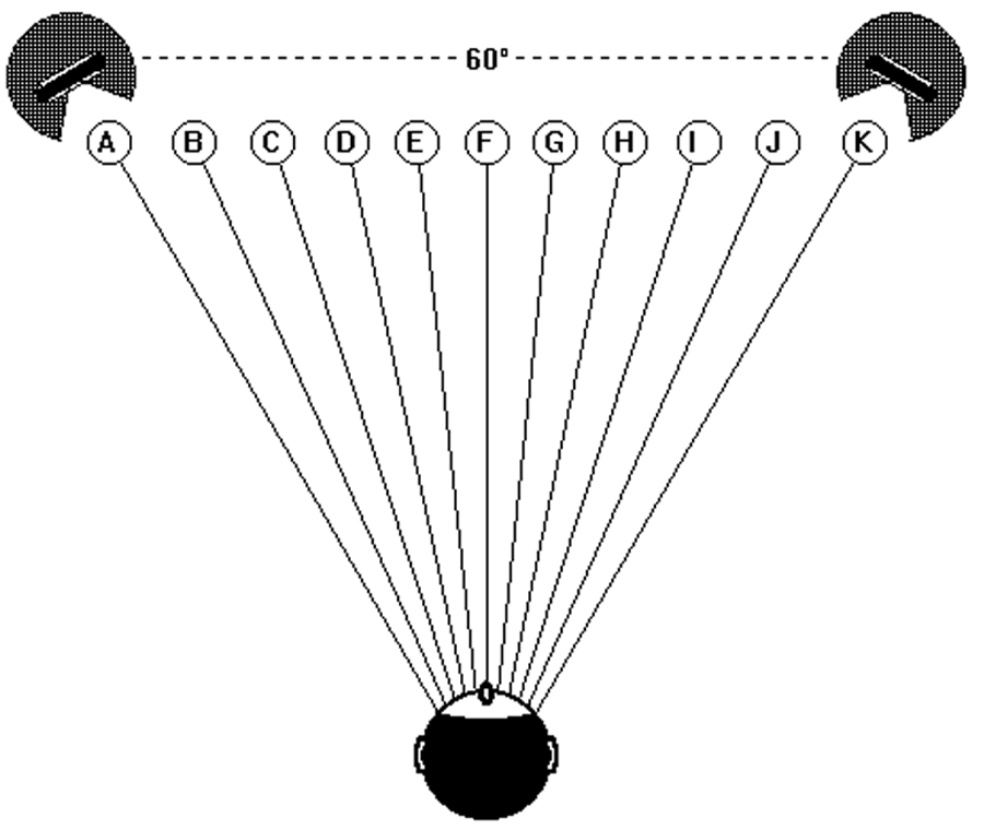Figure 12 – Angular expansion in reproduction (but without angular distortion)

Angular Distortion is one of the operational limitations to the choice of various combinations of distance and angle in the SRA diagrams. It can vary considerably in relation to the directivity pattern that is chosen. In general, it would seem normal to choose combinations that present a minimum of Angular Distortion, but of course, certain sound recording situations can warrant the use of higher values of Angular Distortion. The sound recording engineer must have a wide knowledge of all the characteristics of the different systems available in order to be able to choose the system that will be absolutely optimum in a given situation.

On each SRA diagram, specific values of Angular Distortion are shown in boxes situated along each SRA curve. These values should give an idea of the relative quantity of Angular Distortion. To understand the significance of a specific Angular Distortion value we need to look a bit closer at the way these values were derived. In Figure 13, we have a series of sound sources A, B, C, D and E, situated at equal distances along the arc of a circle.

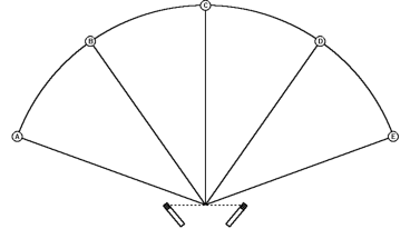Figure 13 – Five sound sources A, B, C, D and E at regular angular spacing

If no Angular Distortion exists in reproduction, then the relative positions of A, B, C, D and E will be maintained (Figure 14).

• A at the left-hand loudspeaker

• B midway between left loudspeaker and centre

• C in the centre

• D midway between right loudspeaker and centre

• E at the right-hand loudspeaker

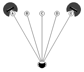Figure 14 – No angular distortion with reproduction

Angular Distortion will modify the reproduced positions of sound sources B and D, they will be shifted towards each loudspeaker, as illustrated in Figure 15, where a shift of 5° of B and D is shown. The sound sources A, C and E will not be affected by this shift and will remain in the same relative position (A and E being, by definition, the limit of the SRA, C being the centre of the system).

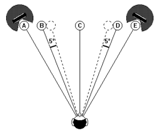Figure 15 – Angular Distortion of 5°

It is this Angular Shift of the sound sources B and D that is used in the SRA diagrams, to represent the maximum Angular Distortion of a given system. We can read off the SRA diagrams specific values of Angular Distortion for given combinations of distance/angle from Figures 8, 9 and 10. Here are a few examples taken from Figure 9 (SRA diagram for cardioid microphones):

               15 cm 110° >>>>>>>>5° (SRA of ± 50°)

               28 cm 60°  >>>>>>>>4° (SRA of ± 50°)

               0 cm 90°   >>>>>>>>6° (SRA of ± 90°)

               37 cm 0°    >>>>>>>>9° (SRA of ± 80°)

This characteristic of Angular Distortion is perceived as a compression or crushing of the extremities of the reproduced sound field towards the loudspeakers. This can also be interpreted as a stretching of the centre of the reproduced sound image, sometimes called “hole in the centre”. This is in fact a misnomer, as the centre of the sound image still exists but is distributed over a wider sector.

It should be noted that in Figure 9, for example, the Angular Distortion is minimal towards the centre of the diagram. In other words, for a given SRA, one obtains minimum Angular Distortion by using a combination of Intensity Difference (Angle) and Time Difference (Distance) stereophony in about equal proportions. Angular Distortion increases by a few degrees with systems using only Intensity Difference (Distance = 0cm), and even more so with systems using mostly Time Difference (Angle between microphones = 0° or with spaced omnidirectional microphones).

It is also possible to see from these SRA diagrams how the specific directivity that is chosen for the microphones has an effect on the quantity of Angular Distortion at various combinations of distance/angle. The most extreme case is omnidirectional microphones spaced at 40 cm to 50 cm, where Angular Distortion is about 9° to 10°.

I.4.2  Variation of the ratio of direct to reverberant sound within the Stereophonic Recording Angle

There are two distinct zones, shown in Figures 8, 9 and 10 by shaded areas, where this problem exists. In the shaded area at the top of each diagram, the ratio of direct to reverberant sound decreases towards the CENTRE of the SRA, whereas, in the shaded area at the bottom of each diagram, this ratio decreases towards the EXTREMITIES of the SRA.

This effect is obviously more apparent in reverberant surroundings, and can to some extent be neglected in a relatively “dead” studio environment. In an outside recording, however, the reverberation level is replaced by the environmental ambience and these zones may again become apparent.

The exact angle at which change in reverberation becomes unacceptable is again a subjective factor and can vary from one person to another. The limits shown on the diagrams can again only be an approximation.

I. 5  Recording procedure

We are now ready to put into practice the Variable Dual Microphone System in a stereophonic recording situation. Good angular localisation of the reproduced stereophonic image plays an important role in stereophonic sound recording. It is certainly not the only factor that must be considered, but it is one of the most important. In what order should one analyse each of the parameters of the microphone system in relation to the characteristics of the sound source and its acoustic environment?

• Frequency Response Curve of the microphones

• Position of the microphone system

• Localisation within the Stereophonic Sound Image

Here again, each sound recording engineer must use his or her own knowledge and judgement to adapt to circumstances, and of course, each person may have individual preferences. It would also be a mistake to try and standardise a given procedure, just as much as it would be a mistake to try and pass on one’s own individual way of working – this leads sooner or later to a complete sclerosis of the “art of sound recording”.

The following procedure should therefore be considered just as a starting point (if this is needed), in developing your own working methods:

1) Frequency Response Curve

Each microphone has a typical frequency characteristic which determines the quality of timbre reproduction of the sound source. This characteristic, especially with respect to the bass response, must be considered in relation to the directivity of the microphones to be used as shown in Figure 7.

2) Position of the microphone system

Here we are looking for the optimum ratio of direct to reverberant sound, as well as a good balance between individual elements of the sound source. If these two factors are not compatible, it is here that perhaps the first compromise has to be considered.

3) Stereophonic Sound Image

The Stereophonic Recording Angle is chosen so as to take into account the sector occupied by the sound source, plus any “sideroom” that is considered necessary.

4) Angular Distortion

In general, there is but one combination of distance/angle for the desired SRA, if minimum Angular Distortion is required. Otherwise, the only restriction in the choice of other combinations of distance/angle is that the shaded areas should be avoided, unless specific effects are considered necessary.

5) Mono/Stereo computability

The different combinations of distance/angle available enable one to opt for Intensity Difference Stereophony (having good mono/stereo compatibility) or, on the other hand, to increase the Time Difference contribution to obtain a better feeling of “space”, but we all have different ideas on this subject!

If a specific characteristic is causing difficulty, it may be necessary to change the order of priority and start this sequence again. This process continues until optimum results are obtained or at least, the best possible compromise.

I. 6 Measuring instruments

The sector, occupied by the sound source plus any sideroom that is desired, must be determined reasonably accurately so that one can read off from the SRA diagrams the combinations of distance and angle for the required Stereophonic Recording Angle. At present, no measuring instrument exists that is adapted to this type of measurement, except perhaps the sextant. This situation is easily rectified if you are prepared to take up a saw, hammer, and nails, and follow a simple “Do It Yourself” plan.

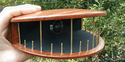
The optical part of the instrument that will be described is a 180° optical viewer (“Judas hole”), normally mounted as a door viewer, to check who is outside before opening up. In France, one of the firms making this viewer is called “BLOSCOP”, however, there must exist a number of firms making this type of device in other parts of the world. It is worth buying the luxury model with maximum diameter optics in order to obtain a good clear image and a real 180° viewing field. You could also use the “Fish Eye” lens from your camera as a viewer, but this is a rather expensive solution to the problem.

The details of the complete viewer are shown in Figure 16, and as you can see, the only materials that are needed are a few long and short nails and some off-cuts of plywood. Nails have been placed every 10°. The long nails are placed at 0°, ± 30° and ± 60°.

Measuring the sector covered by the sound source is now a simple matter of looking at the sound source through this viewer and reading off the angle corresponding to the left and right limits of the sound source. Figure 17 shows such a view through the viewer – you can see why we have nicknamed the instrument “the crocodile”:

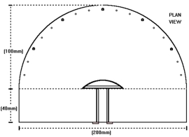
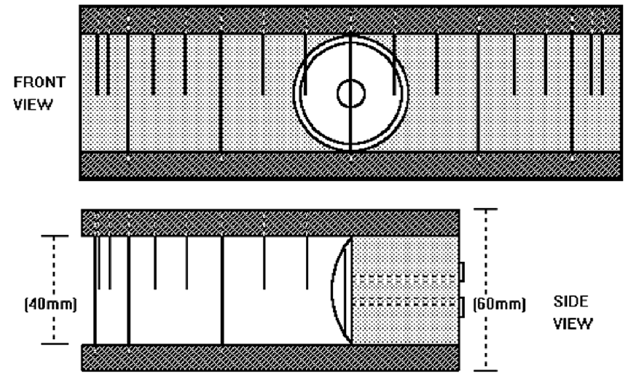Figure 16 – “The Crocodile”

But it is not yet time to leave the workshop, we still need to make a support for the microphone system, so that it is possible to easily adjust both distance and angle between the microphones.

A metal bar in Duralumin or other similar metal of about 300mm long, 25mm wide and 4mm thick must be drilled with 10mm diameter holes every 20mm. The centre hole can be drilled at 8.5mm diameter and threaded with a 3/8″ Whitworth tap if this is available. The bar can then be screwed directly onto the top of a microphone stand. It is now a simple matter to fix two microphone clips at various positions along the bar, using obviously short 3/8″ Whitworth fixing screws to hold the base of the microphone clips. This same thread is often used with photographic equipment, so see whether your local photo shop can help with the necessary fixing screws.

Figure 17 – “The crocodile’s eye view !”

Measurement of the angle between the microphones can be made with a large protractor. But if you can have access to a metal turning lathe, then it would be even better to make a pair of graduated rotating supports for the microphones. The distance between the microphones is measured of course, with a ruler or tape measure.

However, there is a very simple way of setting up the distance and angle between the microphones which requires only a sheet of A4 paper and relies on the ancient Japanese art of “Origami” (but in a very much simplified form)! Here are a few illustrations:

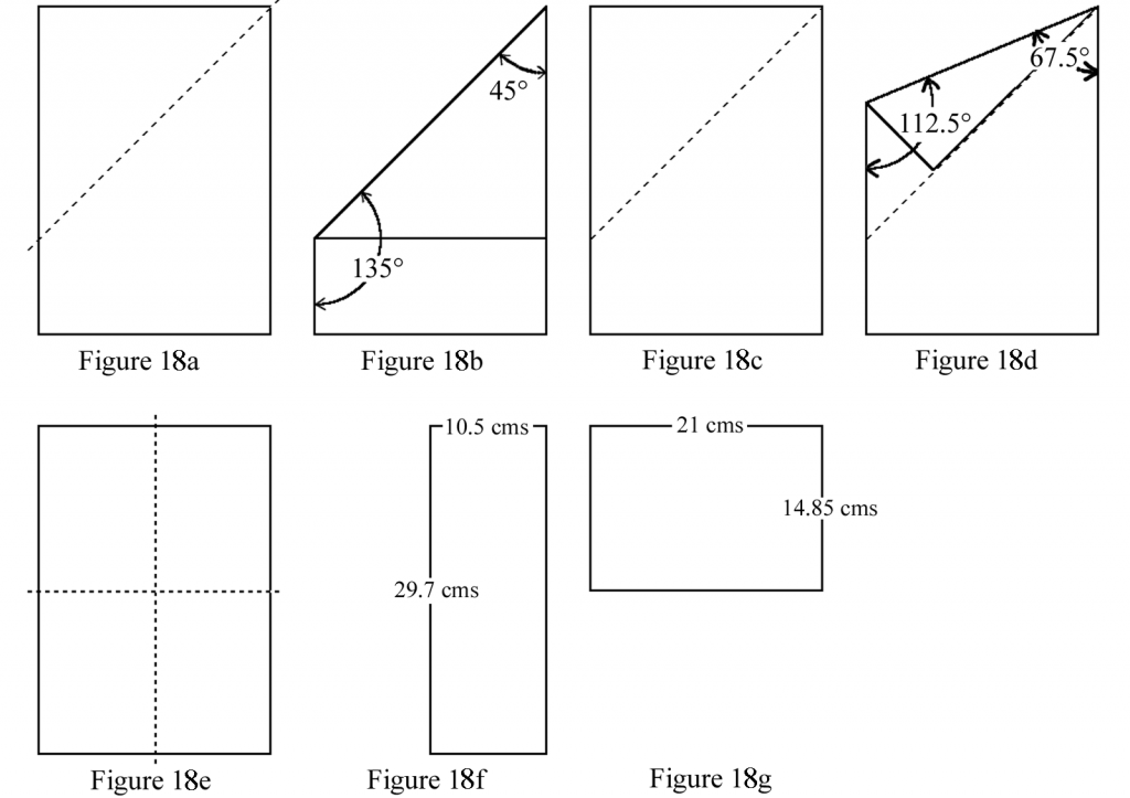Figure 18 – Microphone measurement by “origami”

The corner of an A4 page folded as in Figure 18b will give us 45° and 135°, opened out flat and then folded again as in Figure 18d will give 67.5° and112.5°. This means we can now measure accurately angles of 45°, 67.5°, 90°, 112.5° and 135°, and other angles can be estimated “by eye”. An A4 page (21 cm x 29.7 cm) folded vertically as in Figure 18f will give us a width of 10.5 cm, opened out flat and then folded horizontally as in Figure18g will give us 14.85 cm. So we can measure 10.5 cm, 14.85 cm, 21 cm and 29.7 cm. Again other distances can again be estimated.

7.1 Preliminary listening tests

Before trying to analyse the Variable Dual Microphone System in a real recording situation, it is worthwhile carrying out a few simple listening tests, which will help in your understanding of the basic characteristics of the system. Record someone talking whilst moving along the circumference of the circle of about 1.5 metres in radius. It is important for them to indicate their position in relation to the front axis of the microphone system at about every 10°. The object of the exercise is to try and determine that sector of the angular movement that is reproduced as a stereophonic image between the loudspeakers. The limit of the Stereophonic Recording Angle is obviously the angle at which apparent movement ceases, i.e., when the reproduced sound remains fixed at one or the other of the loudspeakers.

The average voice has a relatively limited frequency range (150Hz to 8kHz), so in order to test the performance of the recording system at frequencies above 8kHz, one must use a different sound source much richer in the higher frequency range (“maracas” or something similar), again indicating every 10° the position of the sound source in relation to the axis of the system. However, it should not come as any surprise to observe that the range of frequencies covered by the human voice will be enough to establish perfectly reliable localisation characteristics. In this way the major part of the characteristics of the microphone system can be analysed.

Here are a few examples of interesting combinations of distance and angle that can be tried using cardioid microphones to start with:

a)  0 cm 90°   } Coincident cardioid

b)  0 cm 180°  } Intensity difference

c)  0 cm 130°  } Stereophony

d)  0 cm 60°   }

e)  30 cm 90°  } Spaced cardioid

f)  20 cm 70°  } Intensity and time difference

g)  10 cm 60°  } Stereophony

h)  35 cm 10°  }

Note carefully your impressions during these listening tests, with special reference to:

• Perceived Stereophonic Recording Angle

• Impression of Angular Distortion

• Evolution of the ratio of direct to reverberant sound within the SRA

• Precision of the reproduced sound image

• Spatial impression

Not only will this type of critical listening test help in your knowledge of the various combinations that can be used in the Variable Dual-Microphone System, but it can help considerably in the basic training of the ear to analyse the different characteristics of a stereophonic recording.

I. 7.2  Experimental recording and listening tests

For the sake of this specific type of test it is interesting to divide the sound sources into four categories:

1. Straight-line moving sources.

A very common type of sound: a passing train, car, motorbike, a plane taking off or landing, footsteps passing from one side to another, etc…..

2.  Continuous straight-line sources.

The sound source is spread out in a straight line from left to right: waves on a beach.

3.  Sound sources occupying an angular sector less than 180°.

This is the most common situation encountered in everyday recording: an orchestra, a group of people in conversation, a firework display at a certain distance, chickens in a field or chicken coop!!!….

4.  Totally surrounding environmental sounds: This is probably the most difficult type of sound to reproduce as the reproduction sound stage is limited to only 60°. Birds in a forest, noises and conversation in the middle of a market, the ambience in a railway station, etc…

Each of these types of sound source has specific sound recording difficulties and requires a different approach to obtain satisfactory reproduction. The different SRA diagrams (Figures 8, 9 and 10) enable us to experiment with different possibilities of SRA. The correspondence of each combination tried must be carefully noted in relation to each recording for future reference. A series of listening tests carried out after such recordings, together with a discussion of the results, will often suggest a new series of recordings that are necessary to find the optimum characteristic of SRA for a particular situation. Experimentation with different combinations of distance and angle for the same SRA value can also help in finding the optimum solution for recording that particular sound source and in that specific sound source environment.

The “quality” of stereophonic reproduction can also vary considerably according to the type of sound source used. Musical instruments, percussion instruments such as drums, xylophone or marimba, with little decay time, should be compared with others such as bells or gongs, with a long decay time. The amount of reverberation can also influence the perception of stereophonic “quality”, or is it just that our perception of the timbre of the instrument has changed in this case?

8  Listening with headphones

Unfortunately, it is quite often necessary to monitor a stereophonic recording using headphones, even though the recording will eventually be heard on loudspeakers. The characteristics of the sound image (SRA, Angular Distortion, etc.) heard on headphones will differ considerably from that reproduced by loudspeaker stereophony. There is no simple solution to this problem, except to use the headphones to monitor only the technical quality of the signal together with the ratio of direct to reverberant sound and rely on the angular measurements made with the “crocodile” as a basis on which to choose the Stereophonic Recording Angle. This problem with headphones is as simple to understand as it is complex to solve. When using a pair of headphones, one hears only the left channel with the left ear and vice versa, this is normally called Binaural Stereophony. On the other hand, when listening to loudspeaker stereophony, the left ear hears both the left and the right loudspeaker, the latter being heard with a certain attenuation. Similarly, the right ear hears both right and left LS signals, with the left LS signal slightly attenuated.

This acoustic interference of the left loudspeaker source on the sound received by the right-hand ear, and the right source on the left ear, is called “Acoustic Crosstalk”. In order to obtain a satisfactory stereophonic sound image with loudspeakers, it is necessary to about double the Intensity Difference and Time Difference in relation to the quantity necessary to produce a good sound image with headphones. This means that a good stereo image on headphones will be too small in the loudspeaker base or sound stage – the sound image will be situated towards the centre of the loudspeaker baseline. Whereas a good loudspeaker stereo image, will be much too wide for headphones – the sound will seem to be just on the left and right ear, with little in between.

There is, however, a way of passing from one listening situation to the other. It is necessary to transform the analogue audio signal into digital information, and by the techniques of Digital Signal Processing reduce the effect of crosstalk. But this process is at an early stage in its development and we will have to wait a few years before it becomes available as a standard correction to the type of listening system used.

9 Analysis of the listening tests

The original text of this document was first published in 1989 in France, as a series of articles published every two months for the magazine called “Actualité de la Scénographie”. At the time, we thought it a worthwhile experiment to try and persuade the readers to carry out the recording and listening tests without having any information concerning what they were supposed to hear, and the actual analysis of the listening tests followed two months later in the next edition.

Our reasoning behind this method of presentation was very simple. It is very difficult to create a neutral listening situation, our capacity to analyse a sound image is too often influenced by intellectual considerations or simply by the visual environment. In other words, if we know what we want to hear or what we should hear, then we are quite capable of persuading ourselves that that is exactly what we are hearing!

This is a problem in everyday work even with the most experienced sound recording engineers and is even worse in the case of students learning. In their eagerness to succeed the student will adopt any visual or intellectual clues that are available, completely missing the one and only factor that is important, which is their own listening experience.

It is the duty of the instructor to eliminate all the visual clues and create the conditions necessary to stimulate real listening.

This article is an extract from the first chapter of the original publication “St Zoom” by Michael Williams and should enable the sound recording engineer quickly to use the St Zoom System for everyday sound recording with a minimum of study.

However, it must not be forgotten that a deeper understanding of the operational method and its justification must take into account a detailed mathematical, physical, and psychoacoustical analysis of the characteristics of the stereophonic microphone system. This subject is developed in the second chapter of the book “St Zoom”, the third chapter being an attempt to reply to the numerous questions that arise concerning the basic theory involved in the development of the system and the application of this system of stereophonic sound recording to the multitude of situations encountered in everyday recording.

The complete document can be obtained from Michael Williams, “Sounds of Scotland”, BP50, 94364 BRY SUR MARNE CEDEX, France or by email: soundsscot@aol.com

Michael Williams started his professional career at the BBC Television Studios in London in 1960. In 1965, he moved to France to work for ”Societe Audax” in Paris developing loudspeakers for professional sound and television broadcasting, and later worked for the ”Conservatoire National des Arts et Metiers” in the adult education television service. In 1980, he became a freelance instructor in Audio Engineering and Sound Recording Practice, working for most of the major French national television and sound broadcasting companies, as well as many training schools and institutions. He is an active member of the Audio Engineering Society and has published many papers on Stereo and Multichannel Recording Systems over the past twenty years. He is at present the AES Publications Sales Representative in Europe.

Originally published in 2010 by Microphone Data Ltd

© 2023 Micpedia