The interpretation of the microphone data sheets

By Michael Williams

Introduction

Despite the remarkable choice of signal processing equipment available in the present-day sound recording studio, the choice of a microphone by the sound recording engineer is still of fundamental importance in determining the final quality of a recording. This choice must be based on a good knowledge of the technical specifications of the microphone as well as a wider operational experience with different sound sources and recording environments.

Before the publication of “Microphone Data” by Rycote (originally in book form, then on CD-ROM, and now online as Micpedia), the assembling of all the data concerning different microphone specifications was no mean task. In fact, in some cases, it was doubtful even if manufacturers really wanted their customers to read and understand these specifications! The publication of this data by Micpedia in a formalised and neutral format is a major advance in helping the sound recording engineer to make a reasoned choice of a microphone for a particular usage. In most cases, this information must be used in conjunction with the more subjective appreciation of sound quality transmitted by the microphone under operational conditions. However, nothing can replace the initial selection based on a comprehensive analysis of the basic specification of the microphone.

In the many years that I have been teaching sound engineering and sound recording practice, the analysis of microphone specifications has been a necessary stage in the training process, enabling the student to make his own reasoned choice of a microphone for a specific sound recording situation, and also helping to contribute to his general background knowledge of “the tools of the trade”. Unfortunately, this training process is usually a constant battle against information coming from a flood of articles in various magazines and even in some books, in which authors give their particular solution to a given recording situation, choice of microphone, position, etc. This type of publication would seem initially inoffensive or even informative, but in reality, is highly counterproductive. The student and even, unfortunately, some experienced sound engineers, will too easily rely on these published “recipes”, rather than developing their own personal judgement.

It is the development of one’s own artistic judgement that is responsible for creating a certain originality or character in the eventual sound quality, upon which, our future career depends. Even the instructor himself must resist passing on his own preferences to the student so as to force him into making his own decisions based on good scientific data and personal on-site operational experience. This training is, of course, an ongoing process. The surest guarantee for the future of quality sound recording is in the continued experimentation at every possible stage of the recording process. Unfortunately, the economic pressures reducing the time available for experimentation are always present. However without this experimentation, especially with all the new technologies available, the fascinating “métier” of the sound recording engineer can but sink into mediocrity.

Anyway, that is enough of the philosophy, back to the job at hand! All credit to Rycote and Chris Woolf, the editor, for their effort in the presentation of the microphone data. In respecting the now international standards for the specification of the different characteristics of a microphone they have at last brought a certain degree of uniformity to all the available information. However the uninitiated should still be forgiven for thinking that these characteristics remain rather difficult to integrate into the practical world of sound recording. There are very good reasons for the form in which each of these characteristics is specified. But an overall view of these characteristics, enabling one to make an intelligent comparison between microphones, still remains rather difficult.

However, you should not be surprised to hear that any improvement in understanding the interpretation of these specifications also needs some additional effort by the reader. The effort to be made is, wait for it – is in the use of “logarithms” and “decibels”. But we are thankfully far from the days of logarithm tables and slide rules. So nobody should refuse the simplicity of hitting a few buttons on a calculator to get this microphone data jargon into a more understandable form. And please don’t blame Rycote for not transforming the microphone data, remember they have used the international standard format for each characteristic within the specification of a given microphone, as supplied by the manufacturers. For the time being, it is therefore up to the user to transform this information, according to his needs.

We need to know the general sensitivity of the microphone and how this will relate to the input stage of, for instance, the mixing desk. We also need to know the total dynamic range within which we can position the dynamic of the sound source. This second characteristic obviously implies knowledge of both the maximum sound level that can be accepted by the microphone and transmitted to the next stages of amplification and of course the noise floor of the microphone. With the advent of digital technology, we now have available a remarkable dynamic range within which we can record. This does not however exempt us from the need for careful matching of the dynamic range of the sound source transmitted through the microphone to the mixing desk, to the various processing equipment and eventually to the recording media.

Headroom must still be allowed for, in order to accommodate unexpected high-level signals, and the very low signal levels must obviously be well above the general noise floor, be it acoustic noise in the studio, electric noise generated by the microphone or the mixing and processing equipment, or simply the noise floor of the recording medium. In some cases, the noise floor can even be determined by a specific listening environment such as the automobile!

Sensitivity

The starting point for this series of calculations is the “Output Sensitivity” of the microphone. The “Output Sensitivity” measurement indicates the level of electrical signal that will be produced by a specific microphone in the presence of a standard acoustic stimulus – it is the key link between the acoustic domain and the electrical domain. This measurement is normally specified as the number of millivolts generated by the microphone when the capsule of the microphone is subjected to an acoustic pressure of 1 Pascal. This value is shown in the data sheets in:

mV/Pa

This is the standard convention that has been adopted by Rycote in the presentation of the microphone data sheets.

There are various other measurement units that can be used to express the level of reference sound pressure used for the “Output Sensitivity” measurement. For instance, the acoustic pressure value of “1 Pa” can also be expressed as a Sound Pressure Level of “94dB SPL”. “Sound Pressure Level” is calculated with respect to a reference acoustic pressure of 2 x 10-5 Pa. This is considered to be the average threshold of sensitivity of the ear at 1000 Hz.

An acoustic pressure of:

1 Pa = 20 Log (1 / 2 x 10-5) = 94 dB SPL

1 Pa of acoustic pressure is also equivalent to “10 µbars” or “10 dynes/cm2”, but nowadays the measurement units of “Pascals” and “dB SPLs” are by far the most frequently used.

If you compare Micpedia’s data presentation with commercially available microphone specification sheets, you will see that some manufacturers still specify the output sensitivity measurement with respect to a standard acoustic stimulus of “1 µbar” (0.1 Pa) which corresponds to 74 SPL (i.e. an acoustic pressure some 20 dB lower). In this case, the output sensitivity will be shown as:

mV/µbar

Other measurement units can also be used to express the value of the electrical output signal. The output voltage from the microphone can be expressed in “decibels” with respect to a reference voltage (Vref) value using the formula :

Output Sensitivity in decibels = 20 log10 (Vm / Vref)

where Vₘ is the Output Sensitivity Voltage of the microphone.

This reference value (Vᵣₑ𝒻) of 0 decibels (0 dBm) is normally accepted as “775 mV into a load of 600 ohms” (or 0dBu if the termination impedance is disregarded). However, this reference value can also refer to “1 volt into a load of 1000 ohms” in which case the suffix is dBV.

However, in Micpedia’s presentation of the microphone data sheets, all sensitivity values are expressed as:

mV/Pa

If we take an electrostatic microphone with a typical sensitivity of about 7.75mV/Pa as an example, we can establish the correspondence between the other measurement units, be it in the acoustical or electrical domain. In this example:

An acoustical stimulus of 1 Pa or 94 dB SPL will produce an electrical output of

7.75 mV or  -40 dBu

This can be compared with the typical sensitivity of a moving-coil electro-dynamic microphone of about 0.775 mV/Pa :

1 Pa or 94 dB SPL will produce

0.775 mV or -60 dBu

This shows that the “dynamic” microphone is about 10 times or 20 dB less sensitive than the “static” microphone. Click through some model pages on Micpedia and compare the sensitivity values of different types of microphones. The transformation of a few “mV/Pa” into “dBu” would also be a useful exercise.

This calculation of “Output Sensitivity” in both the acoustical and electrical domain and in the various measurement units, will help us to “position” the other microphone characteristics such as “noise floor” and “Maximum Sound Pressure Level”.

Maximum sound pressure level

“Maximum SPL” is an indication of the maximum high-level acoustic sound pressure that can be transformed by the microphone into an electrical signal before the onset of distortion. This distortion can be due to either the physical limitations of the capsule or the initial amplification stage within the microphone. Unfortunately, the “Max SPL” as expressed by each manufacturer is not always made within the same set of measurement conditions. As explained by Chris Woolf in his guide to Micpedia (paragraph “Max SPL” of “What the fields mean”), it is important to verify the “percentage of distortion” at which this “Maximum SPL” is measured, as different manufacturers will specify a different percentage of Total Harmonic Distortion levels for the measurement of Max SPL, and, in many cases, do not indicate any %THD value at all!

For high-quality studio microphones, a value of 0.5% THD would seem to be an acceptable common denominator. As suggested by Chris Woolf, for THD values specified for 1% THD, an approximation to 0.5% THD can be obtained by reducing the Max SPL specified by 6dB. Although this is a useful rule of thumb when comparing specifications, it must be borne in mind that the precise value of distortion will be dependent on the specific transfer function of the microphone. For microphones without any indication of %THD in the measurement of Max SPL, the user would be excused for assuming that the Max SPL specified is just before “drastic clipping”. Let us hope that manufacturers can be persuaded to be more explicit in their specifications. For instance, measurement at two values of THD (0.5% and 2%) might clarify the situation for most users.

Obviously, the origins of this distortion will differ considerably depending on the type of microphone under consideration. In fact with electro-dynamic microphones, whether moving coil or ribbon, the “maximum SPL” is usually not even specified. Except for electro-dynamic microphones used in very special circumstances, this characteristic is therefore only of interest in the analysis of the performance of electrostatic microphones.

Our transformation of this “Max SPL” value is again a process of establishing the correspondence between all the different measurement units, be it in the acoustical or electrical domain. This time, as the characteristic is expressed in “Pascals”, we
need to establish the equivalent value in “SPLs” in the acoustical domain, and in “mV” and “decibels” in the electrical domain, in order to have an overall view.

Let us take as an example a “Max SPL” value of “100 Pa”. This is some 100 times, or 40dB, greater than the standard acoustic stimulus value (1 Pa or 94 dB SPL) for the measurement of output sensitivity. “Max SPL” could therefore also be specified as 134 dB SPL (94 dB SPL + 40 dB). This value can also be expressed in the electrical domain. The output voltage generated by this high-level acoustic stimulus will also be 100 times greater, or 40dB above, the output sensitivity value. If this microphone has an “Output Sensitivity” of 7.75mV/Pa or -40 dBu/Pa (the example used previously), the “Max SPL” would generate an output voltage of 775mV, or 0 dBu. This is clearly shown in the following diagram:

Max SPL	100 Pa	=	134 dBSPL		775 mV		0 dBu
	↑		↑		↑		↑
	multiply by 100		40 dB		multiply by 100		40 dB
	|		↓		|		↓
Output sensitivity	1 Pa	=	94 dB SPL	>>>	7.75mV/Pa	=>	-40 dBu

It is now a simple matter to check the specification of the next amplification stage to see if it will accept such a voltage level without generating distortion.

---

The noise floor

In Micpedia’s presentation of data, the specification of the noise floor is called “Self  Noise”, i.e., the noise generated by the microphone system. In practice, this is applicable to the noise generated by the capsule and any internal amplification system incorporated into the microphone housing, usually the microphone preamplifier.

It is unfortunate that the use of only this definition of the noise floor excludes the measurement of noise induced in the microphone capsule construction due to surrounding magnetic fields – typically mains induced 50/60Hz “hum”. This characteristic is, of course, of particular interest in the construction of a quality moving coil or ribbon electrodynamic microphone.

All microphones have a self-noise level, that is, an electrical output when no appreciable sound is present. In electrodynamic microphones, this is the sum of noise generated by random air particle movement near the diaphragm, as influenced by the diaphragm loading, and the noise generated by thermal agitation in the voice coil or ribbon, and transformer. In some ribbon microphones, this noise is quite a bit higher than the noise from all sources generated in a condenser microphone. In modern condenser microphones, the dominant noise floor is no longer from the electronics but rather from the air both in front of the diaphragm and the trapped air cushion damping the diaphragm movement. Noise from the amplifier is also present but is seldom the main source.

The “Self Noise” generated by an electrostatic microphone is normally expressed as “an equivalent acoustic noise value”. In other words, the level of acoustical stimulus that will produce an electrical signal equivalent in the microphone to the electrical noise generated by the microphone. This is obviously a good representation of the noise floor of the microphone when making a comparison with the acoustic noise level in the studio or with the lower end of the dynamic range of a musical instrument or other types of sound source. However, this does not help us to position this lower limit of the dynamic range in relation to the following amplification stages in the recording chain. So again we must transform this “Self Noise” value into other useful measurement units in the acoustical and electrical domain.

The subjective impact of noise also depends very much on the eventual level at which the noise is heard. Low-level noise will not create the same subjective impression as noise at a higher level. In particular, our reduced perception of low-level noise in the bass frequency range (as shown by the psychoacoustic measurements of hearing sensitivity published by Fletcher & Munson, Dadson & King, ….) would seem to indicate that the CCIR-468 measurement of the “Self Noise” characteristic would be more appropriate to basic operational conditions, as it is a good approximation to the reception curve of the human ear at very low sound pressure levels. The DIN/IEC “A-weighting” measurement (dB-A) measurement is closer to hearing reception at levels of about 40dB SPL or more correctly 40 phons. However, both the CCIR and the DIN/IEC specification of “Self Noise” have been supplied by certain manufacturers.

There is an international standard, IEC 60268-4, that applies to microphone performance characterisation in general, unfortunately, none of the microphone manufacturers at present provide specifications that are compliant with this standard. It would seem that this is not for lack of the ability to make the measurements, but rather a lack of consensus on how to present this information to the public.

Again we must transform the specification of this specific characteristic into our usual set of measurement values in the acoustical and electrical domain.

Let us consider that our example microphone has a “Self Noise” value of “14 dB SPL”. This is 80 dB lower than the standard acoustic stimulus value for the measurement of output sensitivity, or 10000 times lower than 1 Pa i.e. at 10-4 Pa. So we would expect the output voltage of self-noise from the microphone also to be some 80dB below the output sensitivity value, or 10000 times less. The “Output Sensitivity” of our example microphone is 7.75mV/Pa or –40 dBu/Pa, therefore the “Self Noise” voltage would be:

0.775µV (7.75mV divided by 10000)

or

-120 dBu (-40 dBu minus 80 dB).

This is shown clearly in the following diagram.

Output sensitivity	1 Pa	=	94 dBSPL	>>>	7.75 mV/PA	=>	-40 dBu
	|		↑		|		↑
	divide by 1000		80 dB		divide by 1000		80 dB
	↓		↓		↓		↓
Self Noise	10⁻⁴ Pa		14 dB SPL	>>>	0.775 μV	=	-120 dBu

---

From the calculated values of “Max SPL” and “Self Noise” used in the above example we can now see that the dynamic range of this “fictional” microphone is:

Dynamic Range = (Max SPL) – (Self Noise in SPL)
= 134 dB SPL – 14 dB SPL = 120 dB

The values chosen for all these examples have been selected so as to simplify the calculation as much as possible. Real-life values will obviously not be so considerate!

To pilot you through your first set of calculations, I will take as a worked example the microphone “Neumann U87”, after that, you are on your own. The values read from the data sheets are indicated in thin green border boxes. Calculated values are either in italics or bold red border boxes.

The “Output Sensitivity” specified in the Neumann U87 data sheet is:

28 mV/Pa

Output Sensitivity in decibels = 20 log₁₀ (28 / 775) = – 28.8 dBu

So the “Output Sensitivity” line becomes:

Output sensitivity

1 Pa

=

94dBSPL

>>>

28mV/Pa

=>

-28.84 dBu

Max SPL is specified as:

117dB SPL

This is 23dB higher than the reference level for the measurement of Output Sensitivity of 94dB SPL.

117 dB SPL – 94 dB SPL = 23 dB

The start of our Max SPL line is now:

Max SPL			117 Pa
			↑
			23 dB
			↓
Output sensitivity	1 Pa	=	94 dB SPL	>>>	28mV/Pa	=>	-28.84 dBu

There are two ways to find the equivalent value of this SPL in Pa:

Either transform 23 dB into a ratio:

ratio = 10⁽²³ᐟ²⁰⁾ = 14.1

therefore 1 Pa x 14.1 = 14.1 Pa

or transform 117 dB SPL into Pa with respect to the reference O dB SPL of 2 x 10⁻⁵ Pa:

 Max SPL in Pa = (2 x 10⁻⁵ ) x 10⁽¹¹⁷ᐟ²⁰⁾ = 14.1 Pa

The start of our specification chart is now:

Max SPL	14.1 Pa	=	117 dB SPL
	↑		↑
	multiply by 14.1		23 dB
	|		↓
Output sensitivity	1 Pa	=	94 dB SPL	>>>	28mV/Pa	=>	-28.84 dBu

We can use both the ratio of 14.1 and the decibel difference value of 23 dB to fill in the values in the electrical domain.

Max SPL	14.1 Pa	=	117 dB SPL		395.5 mV		-5.84 dBu
	↑		↑		↑		↑
	multiply by 14.1		23 dB		multiply by 14.1		23 dB
	|		↓		|		↓
Output sensitivity	1 Pa	=	94 dB SPL	>>>	28mV/Pa	=>	-28.84 dBu

Self Noise is specified as:

23 dB SPL

This is 71 dB less than the reference level for the measurement of Output Sensitivity of 94 dB SPL.

94 dB SPL – 23 dB SPL  = 71 dB

A difference of 71 dB is equivalent to a ratio of 3548:

Ratio  = 10 ⁽⁷¹ᐟ²⁰⁾ = 3548

We can now add the beginning of the Self Noise line to the specification chart:

Max SPL	14.1 Pa	=	117 dB SPL		395.5 mV		-5.84 dBu
	↑		↑		↑		↑
	multiply by 14.1		23 dB		multiply by 14.1		23 dB
	|		↓		|		↓
Output sensitivity	1 Pa	=	94 dB SPL	>>>	28mV/Pa	=>	-28.84 dBu
	↑		↑
	divide by 3548		71 dB
	|		↓
Self noise	2.8 x 10⁻⁴ Pa	=	23 dB

Both the ratio of Self Noise and the decibel difference can be used to complete the Self Noise line:

Max SPL	14.1 Pa	=	117 dB SPL		395.5 mV		-5.84 dBu
	↑		↑		↑		↑
	multiply by 14.1		23 dB		multiply by 14.1		23 dB
	|		↓		|		↓
Output sensitivity	1 Pa	=	94 dB SPL	>>>	28mV/Pa	=>	-28.84 dBu
	|		↑		|		↑
	divide by 3548		71 dB		divide by 3548		71 dB
	↓		↓		↓		↓
Self noise	2.8 x 10⁻⁴ Pa	=	23 dB	>>>	7.89 μV	=	-99.84 dBu

The total dynamic range is now simply a matter of calculating the number of decibels between the Max SPL and Self Noise values.

Total Dynamic Range = 23dB + 71dB = 94dB

---

The frequency response

For many years the frequency response curve has been our first approach to estimating the way in which a microphone will transform the spectral balance of the sound source. In parallel with this scientific measurement, a vast range of subjective vocabulary based on operational experience has been built up to supplement the limitations of this fundamental measurement. This vocabulary (“dry”, “bright”, “boomy”, “resonant”, “metallic”, etc.) has the advantage of seemingly describing in everyday language the basic characteristics of a particular colouration, but unfortunately suffers from a certain ambiguity in interpretation. But this only serves to illustrate the fact that, at present, we do not have adequate measurement techniques available to characterise this aspect of microphone response.

It would seem that the published frequency response measurement can give us only a basic appreciation of the overall tonal balance. It is probable that we are hoping to obtain too much information from only one type of measurement, and also our knowledge concerning the interpretation of different aspects of this characteristic is still rather rudimentary. Added to this, it is probable that our perception of the overall spectral balance is a combination of many interrelated factors, the on-axis response, therefore, being only part of the story. On-axis response is certainly of fundamental importance, but the off-axis response and its rendition of early reflections and reverberation also plays an important role in our subjective appreciation of the tonal balance. Another important contributing factor would seem to be the temporal frequency response, often called the “waterfall” response. That is the frequency response measured at periods over the few milliseconds after the microphone has received the acoustic stimulus signal. Some interesting work has been done in the past few years by Jackie Green (nee Hebrock) in this type of measurement (see AES preprint 4516 & Paper MAL-09, Conference: AES UK Conference 1998 – Microphones & Loudspeakers).

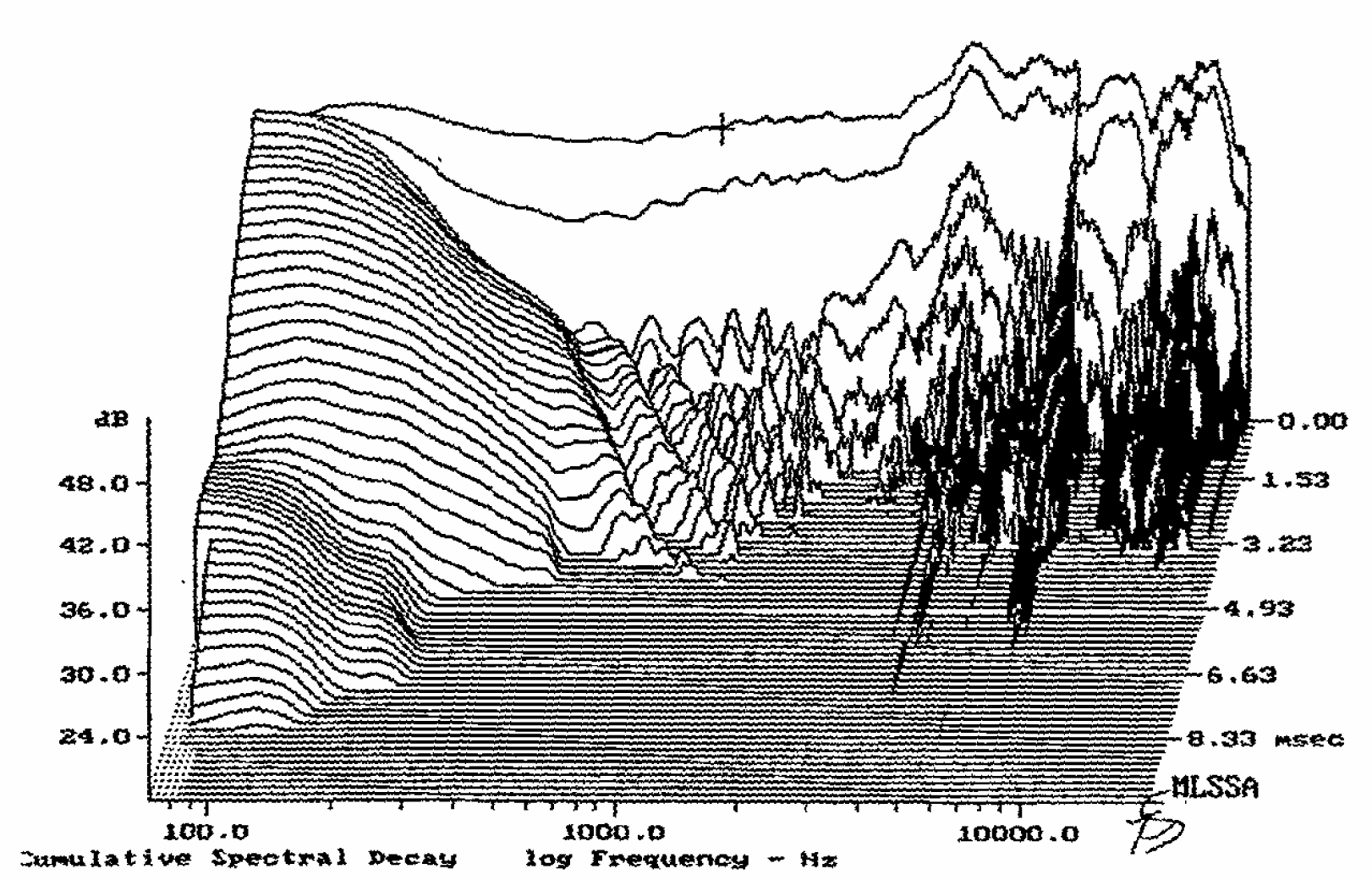
This work would seem to suggest that this “waterfall” type of measurement highlights the various resonances in the microphone response and could go some way to explaining the “colouration” that we hear in some microphones, which is not obvious from the basic frequency response curve. The purists would say that a detailed analysis of the phase response of the microphone should also produce the same type of information. Let us hope that in the future, Micpedia will be able to integrate this type of measurement into its data sheets.

However, the information that can be “read” from a frequency response curve is still a first step in the choice of a suitable microphone for a particular usage, one just has to be conscious of the limitations of this type of measurement for the time being. The low-frequency and high-frequency roll-off (or otherwise) are quite evident, as well as the overall linearity of the response. In hand-held vocal microphones, the amount of proximity effect compensation can also be seen clearly from the frequency response characteristic. However any use of medium frequency range boost to create “presence” must be examined closely, the user should establish his own correlation between the form of the boost that has been applied, and his own requirements or subjective appreciation in operational conditions. And again bear in mind that any typical frequency response curve can always “hide” disagreeable resonances.

One must also be sure that we are reading a “real” response curve of a specific microphone. More often than not, the typical frequency response curve is a hand-drawn mean value with, at best, an indication of tolerance. However, it is in the fine detail that some of the more serious problems can be detected.

Frequency response and the polar diagram

One must pay tribute to the ingenuity of engineers working in the design of microphone systems, to the way they have been able to juggle the many conflicting aspects of microphone design and produce, in general, microphones of such high quality.

Microphone characteristics cannot be considered independent of each other. For instance, there is a fundamental relationship between the low-frequency response of a microphone and its basic directivity pattern. “All other things being equal”, the basic response curve in the low-frequency range of an omnidirectional or pressure microphone is essentially linear and constant, whereas the pure pressure gradient or “figure of eight” directivity pattern microphone has a frequency roll-off of about 6dB per octave towards the low frequencies. It is in the skill of the design of a pressure gradient microphone that a balance is achieved between a reasonable output sensitivity and an acceptable bass frequency response.

Diaphragm diameter also has a direct influence on the directivity pattern of the microphone in the medium and high-frequency range. A relatively constant directivity pattern throughout the audible frequency range can only be obtained with a small diaphragm. However, this can be at the expense of a satisfactory response in the bass frequencies.

Unfortunately, manufacturers seem to devote less and less space to showing us a comprehensive and readable set of polar diagrams. We must content ourselves with a careful inspection under a magnifying glass of these “thumbnail” diagrams in order to bring out the salient points. On Micpedia, we can, however, magnify the diagram on the screen.

The “Specification Chart” for comparison of microphone performance

The calculation of a “specification chart” (as illustrated above) for each individual microphone, facilitates the comparison between the different microphone specifications. The total dynamic range available for each microphone is of course an important factor in the selection process. However, the race for the microphone with the most spectacular specification of dynamic, should not outweigh a balanced appreciation of all the other characteristics.

Matching

The total dynamic range of the sound source must be carefully matched to the microphone’s own dynamic range, and then on to the next amplification stage, usually the input module of the mixing desk. This would seem obvious with respect to the sound source working into a microphone, but the use of the sensitivity adjustment on the input module seems to be still rather intuitive, not to say “haphazard”. Careful consideration must be given to the sensitivity settings of the input module so as to make optimum use of the wide dynamic range available. Too low a sensitivity will need extra amplification at a later stage, and therefore increase the level of the noise floor, whereas too high a sensitivity will increase distortion at high signal levels and may introduce clipping.

Other characteristics

Many microphones are made for a specific type of utilisation, a handheld voice microphone being a common example. This type of microphone, usually pressure-gradient, generally compensates for the proximity effect by a low-frequency roll-off. In addition, the microphone must have some efficient anti-plosive protection and be insensitive to noise transmitted through the microphone housing (handling noise). This type of characteristic although not shown in the Rycote data sheets may possibly be indicated in the short description that accompanies the specification of each microphone.

And of course, another important characteristic is reliability! In the field of outside broadcasting and news gathering, reliability is sometimes more important than any other characteristic. Would it be too much to hope that someday an indication of a microphone’s sensitivity to shock, temperature and humidity could be published? This type of information would probably not go amiss in the studio context also.

Below is a blank specification chart that you can print out to help you with your own calculations.

Michael Williams started his professional career at the BBC Television Studios in London in 1960. In 1965 he moved to France to work for ”Societe Audax” in Paris developing loudspeakers for professional sound and television broadcasting, and later worked for the ”Conservatoire National des Arts et Metiers” in the adult education television service. In 1980 he became a freelance instructor in Audio Engineering and Sound Recording Practice, working for most of the major French national television and sound broadcasting companies, as well as many training schools and institutions. He is an active member of the Audio Engineering Society and has published many papers on Stereo and Multichannel Recording Systems over the past twenty years. He is at present the AES Publications Sales Representative in Europe.

Originally published in 2002 by Rycote Microphone Windshields Ltd and Human Computer Interface for Microphone Data
© 2022 Micpedia

---

Microphone:

Max SPL	_____ Pa	=	_____ dB SPL		_____ mV		_____ dBu
	↑		↑		↑		↑
	multiply by _____		_____ dB		multiply by _____		_____ dB
	|		↓		|		↓
Output sensitivity	1 Pa	=	94 dB SPL	>>>	_____mV/Pa	=>	_____ dBu
	|		↑		|		↑
	divide by _____		_____dB		divide by _____		_____ dB
	↓		↓		↓		↓
Self noise	_____ Pa	=	_____ dB	>>>	_____ μV	=	_____ dBu

Total Dynamic Range =